
diff options
Diffstat (limited to 'content/blog/2020-07-26-business-analysis.md')
| -rw-r--r-- | content/blog/2020-07-26-business-analysis.md | 34 |
1 files changed, 17 insertions, 17 deletions
diff --git a/content/blog/2020-07-26-business-analysis.md b/content/blog/2020-07-26-business-analysis.md index 4105d04..20fb82d 100644 --- a/content/blog/2020-07-26-business-analysis.md +++ b/content/blog/2020-07-26-business-analysis.md @@ -13,10 +13,10 @@ project was obtained using Foursquare's developer API. Fields include: -- Venue Name -- Venue Category -- Venue Latitude -- Venue Longitude +- Venue Name +- Venue Category +- Venue Latitude +- Venue Longitude There are 232 records found using the center of Lincoln as the area of interest with a radius of 10,000. @@ -26,7 +26,7 @@ with a radius of 10,000. The first step is the simplest: import the applicable libraries. We will be using the libraries below for this project. -``` python +```python # Import the Python libraries we will be using import pandas as pd import requests @@ -42,7 +42,7 @@ are using in this project comes directly from the Foursquare API. The first step is to get the latitude and longitude of the city being studied (Lincoln, NE) and setting up the folium map. -``` python +```python # Define the latitude and longitude, then map the results latitude = 40.806862 longitude = -96.681679 @@ -60,7 +60,7 @@ we use our first API call below to determine the total results that Foursquare has found. Since the total results are 232, we perform the API fetching process three times (100 + 100 + 32 = 232). -``` python +```python # Foursquare API credentials CLIENT_ID = 'your-client-id' CLIENT_SECRET = 'your-client-secret' @@ -129,7 +129,7 @@ the categories and name from each business's entry in the Foursquare data automatically. Once all the data has been labeled and combined, the results are stored in the `nearby_venues` dataframe. -``` python +```python # This function will extract the category of the venue from the API dictionary def get_category_type(row): try: @@ -203,7 +203,7 @@ We now have a complete, clean data set. The next step is to visualize this data onto the map we created earlier. We will be using folium's `CircleMarker()` function to do this. -``` python +```python # add markers to map for lat, lng, name, categories in zip(nearby_venues['lat'], nearby_venues['lng'], nearby_venues['name'], nearby_venues['categories']): label = '{} ({})'.format(name, categories) @@ -224,18 +224,18 @@ map_LNK \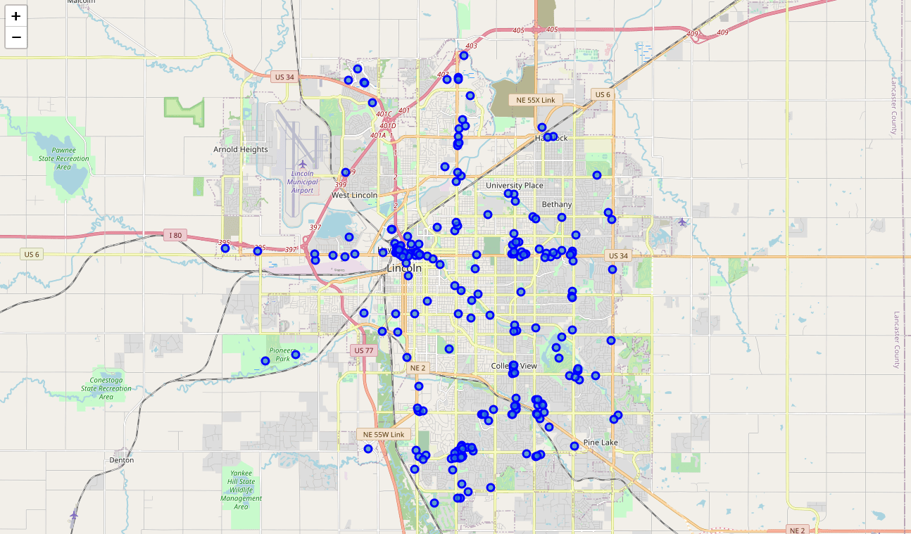 -# Clustering: *k-means* +# Clustering: _k-means_ -To cluster the data, we will be using the *k-means* algorithm. This algorithm is +To cluster the data, we will be using the _k-means_ algorithm. This algorithm is iterative and will automatically make sure that data points in each cluster are as close as possible to each other, while being as far as possible away from other clusters. However, we first have to figure out how many clusters to use (defined as the -variable *'k'*). To do so, we will use the next two functions to calculate the +variable _'k'_). To do so, we will use the next two functions to calculate the sum of squares within clusters and then return the optimal number of clusters. -``` python +```python # This function will return the sum of squares found in the data def calculate_wcss(data): wcss = [] @@ -275,7 +275,7 @@ Now that we have found that our optimal number of clusters is six, we need to perform k-means clustering. When this clustering occurs, each business is assigned a cluster number from 0 to 5 in the dataframe. -``` python +```python # set number of clusters equal to the optimal number kclusters = n @@ -289,7 +289,7 @@ nearby_venues.insert(0, 'Cluster Labels', kmeans.labels_) Success! We now have a dataframe with clean business data, along with a cluster number for each business. Now let's map the data using six different colors. -``` python +```python # create map with clusters map_clusters = folium.Map(location=[latitude, longitude], zoom_start=12) colors = ['#0F9D58', '#DB4437', '#4285F4', '#800080', '#ce12c0', '#171717'] @@ -321,7 +321,7 @@ which clusters are more popular for businesses and which are less popular. The results below show us that clusters 0 through 3 are popular, while clusters 4 and 5 are not very popular at all. -``` python +```python # Show how many venues are in each cluster color_names = ['Dark Green', 'Red', 'Blue', 'Purple', 'Pink', 'Black'] for x in range(0,6): @@ -337,7 +337,7 @@ Our last piece of analysis is to summarize the categories of businesses within each cluster. With these results, we can clearly see that restaurants, coffee shops, and grocery stores are the most popular. -``` python +```python # Calculate how many venues there are in each category # Sort from largest to smallest temp_df = nearby_venues.drop(columns=['name', 'lat', 'lng']) |