
diff options
| author | Christian Cleberg <hello@cleberg.net> | 2024-03-04 22:34:28 -0600 |
|---|---|---|
| committer | Christian Cleberg <hello@cleberg.net> | 2024-03-04 22:34:28 -0600 |
| commit | 797a1404213173791a5f4126a77ad383ceb00064 (patch) | |
| tree | fcbb56dc023c1e490df70478e696041c566e58b4 /content/blog/2020-07-26-business-analysis.md | |
| parent | 3db79e7bb6a34ee94935c22d7f0e18cf227c7813 (diff) | |
| download | cleberg.net-797a1404213173791a5f4126a77ad383ceb00064.tar.gz cleberg.net-797a1404213173791a5f4126a77ad383ceb00064.tar.bz2 cleberg.net-797a1404213173791a5f4126a77ad383ceb00064.zip | |
initial migration to test org-mode
Diffstat (limited to 'content/blog/2020-07-26-business-analysis.md')
| -rw-r--r-- | content/blog/2020-07-26-business-analysis.md | 389 |
1 files changed, 0 insertions, 389 deletions
diff --git a/content/blog/2020-07-26-business-analysis.md b/content/blog/2020-07-26-business-analysis.md deleted file mode 100644 index dd913e6..0000000 --- a/content/blog/2020-07-26-business-analysis.md +++ /dev/null @@ -1,389 +0,0 @@ -+++ -date = 2020-07-26 -title = "Algorithmically Analyzing Local Businesses" -description = "Exploring and visualizing data with Python." -+++ - -# Background Information - -This project aims to help investors learn more about a random city in -order to determine optimal locations for business investments. The data -used in this project was obtained using Foursquare's developer API. - -Fields include: - -- Venue Name -- Venue Category -- Venue Latitude -- Venue Longitude - -There are 232 records found using the center of Lincoln as the area of -interest with a radius of 10,000. - -# Import the Data - -The first step is the simplest: import the applicable libraries. We will -be using the libraries below for this project. - -```python -# Import the Python libraries we will be using -import pandas as pd -import requests -import folium -import math -import json -from pandas.io.json import json_normalize -from sklearn.cluster import KMeans -``` - -To begin our analysis, we need to import the data for this project. The -data we are using in this project comes directly from the Foursquare -API. The first step is to get the latitude and longitude of the city -being studied (Lincoln, NE) and setting up the folium map. - -```python -# Define the latitude and longitude, then map the results -latitude = 40.806862 -longitude = -96.681679 -map_LNK = folium.Map(location=[latitude, longitude], zoom_start=12) - -map_LNK -``` - -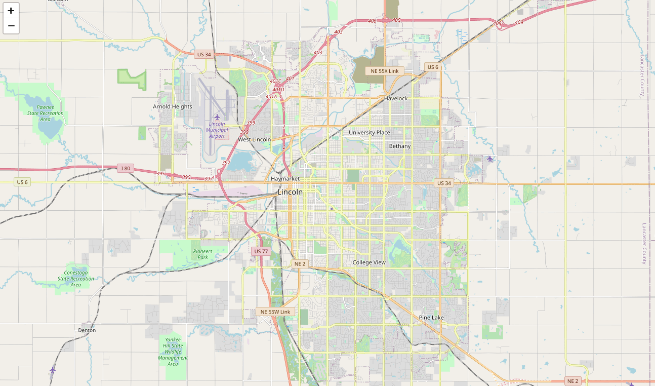 - -Now that we have defined our city and created the map, we need to go get -the business data. The Foursquare API will limit the results to 100 per -API call, so we use our first API call below to determine the total -results that Foursquare has found. Since the total results are 232, we -perform the API fetching process three times (100 + 100 + 32 = 232). - -```python -# Foursquare API credentials -CLIENT_ID = 'your-client-id' -CLIENT_SECRET = 'your-client-secret' -VERSION = '20180604' - -# Set up the URL to fetch the first 100 results -LIMIT = 100 -radius = 10000 -url = 'https://api.foursquare.com/v2/venues/explore?&client_id={}&client_secret={}&v={}&ll={},{}&radius={}&limit={}'.format( - CLIENT_ID, - CLIENT_SECRET, - VERSION, - latitude, - longitude, - radius, - LIMIT) - -# Fetch the first 100 results -results = requests.get(url).json() - -# Determine the total number of results needed to fetch -totalResults = results['response']['totalResults'] -totalResults - -# Set up the URL to fetch the second 100 results (101-200) -LIMIT = 100 -offset = 100 -radius = 10000 -url2 = 'https://api.foursquare.com/v2/venues/explore?&client_id={}&client_secret={}&v={}&ll={},{}&radius={}&limit={}&offset={}'.format( - CLIENT_ID, - CLIENT_SECRET, - VERSION, - latitude, - longitude, - radius, - LIMIT, - offset) - -# Fetch the second 100 results (101-200) -results2 = requests.get(url2).json() - -# Set up the URL to fetch the final results (201 - 232) -LIMIT = 100 -offset = 200 -radius = 10000 -url3 = 'https://api.foursquare.com/v2/venues/explore?&client_id={}&client_secret={}&v={}&ll={},{}&radius={}&limit={}&offset={}'.format( - CLIENT_ID, - CLIENT_SECRET, - VERSION, - latitude, - longitude, - radius, - LIMIT, - offset) - -# Fetch the final results (201 - 232) -results3 = requests.get(url3).json() -``` - -# Clean the Data - -Now that we have our data in three separate dataframes, we need to -combine them into a single dataframe and make sure to reset the index so -that we have a unique ID for each business. The `get~categorytype~` -function below will pull the categories and name from each business's -entry in the Foursquare data automatically. Once all the data has been -labeled and combined, the results are stored in the -`nearby_venues` dataframe. - -```python -# This function will extract the category of the venue from the API dictionary -def get_category_type(row): - try: - categories_list = row['categories'] - except: - categories_list = row['venue.categories'] - - if len(categories_list) == 0: - return None - else: - return categories_list[0]['name'] - -# Get the first 100 venues -venues = results['response']['groups'][0]['items'] -nearby_venues = json_normalize(venues) - -# filter columns -filtered_columns = ['venue.name', 'venue.categories', 'venue.location.lat', 'venue.location.lng'] -nearby_venues = nearby_venues.loc[:, filtered_columns] - -# filter the category for each row -nearby_venues['venue.categories'] = nearby_venues.apply(get_category_type, axis=1) - -# clean columns -nearby_venues.columns = [col.split(".")[-1] for col in nearby_venues.columns] - ---- - -# Get the second 100 venues -venues2 = results2['response']['groups'][0]['items'] -nearby_venues2 = json_normalize(venues2) # flatten JSON - -# filter columns -filtered_columns2 = ['venue.name', 'venue.categories', 'venue.location.lat', 'venue.location.lng'] -nearby_venues2 = nearby_venues2.loc[:, filtered_columns] - -# filter the category for each row -nearby_venues2['venue.categories'] = nearby_venues2.apply(get_category_type, axis=1) - -# clean columns -nearby_venues2.columns = [col.split(".")[-1] for col in nearby_venues.columns] -nearby_venues = nearby_venues.append(nearby_venues2) - ---- - -# Get the rest of the venues -venues3 = results3['response']['groups'][0]['items'] -nearby_venues3 = json_normalize(venues3) # flatten JSON - -# filter columns -filtered_columns3 = ['venue.name', 'venue.categories', 'venue.location.lat', 'venue.location.lng'] -nearby_venues3 = nearby_venues3.loc[:, filtered_columns] - -# filter the category for each row -nearby_venues3['venue.categories'] = nearby_venues3.apply(get_category_type, axis=1) - -# clean columns -nearby_venues3.columns = [col.split(".")[-1] for col in nearby_venues3.columns] - -nearby_venues = nearby_venues.append(nearby_venues3) -nearby_venues = nearby_venues.reset_index(drop=True) -nearby_venues -``` - -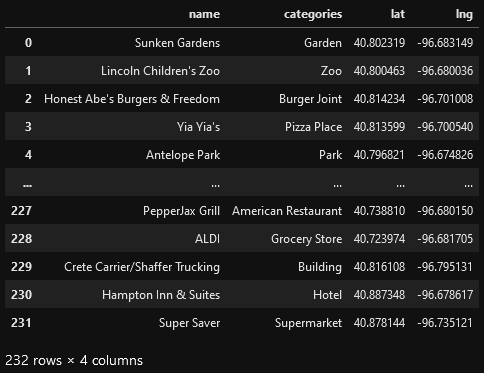 - -# Visualize the Data - -We now have a complete, clean data set. The next step is to visualize -this data onto the map we created earlier. We will be using folium's -`CircleMarker()` function to do this. - -```python -# add markers to map -for lat, lng, name, categories in zip(nearby_venues['lat'], nearby_venues['lng'], nearby_venues['name'], nearby_venues['categories']): - label = '{} ({})'.format(name, categories) - label = folium.Popup(label, parse_html=True) - folium.CircleMarker( - [lat, lng], - radius=5, - popup=label, - color='blue', - fill=True, - fill_color='#3186cc', - fill_opacity=0.7, - ).add_to(map_LNK) - -map_LNK -``` - -\ - -# Clustering: *k-means* - -To cluster the data, we will be using the *k-means* algorithm. This -algorithm is iterative and will automatically make sure that data points -in each cluster are as close as possible to each other, while being as -far as possible away from other clusters. - -However, we first have to figure out how many clusters to use (defined -as the variable *'k'*). To do so, we will use the next two functions -to calculate the sum of squares within clusters and then return the -optimal number of clusters. - -```python -# This function will return the sum of squares found in the data -def calculate_wcss(data): - wcss = [] - for n in range(2, 21): - kmeans = KMeans(n_clusters=n) - kmeans.fit(X=data) - wcss.append(kmeans.inertia_) - - return wcss - -# Drop 'str' cols so we can use k-means clustering -cluster_df = nearby_venues.drop(columns=['name', 'categories']) - -# calculating the within clusters sum-of-squares for 19 cluster amounts -sum_of_squares = calculate_wcss(cluster_df) - -# This function will return the optimal number of clusters -def optimal_number_of_clusters(wcss): - x1, y1 = 2, wcss[0] - x2, y2 = 20, wcss[len(wcss)-1] - - distances = [] - for i in range(len(wcss)): - x0 = i+2 - y0 = wcss[i] - numerator = abs((y2-y1)*x0 - (x2-x1)*y0 + x2*y1 - y2*x1) - denominator = math.sqrt((y2 - y1)**2 + (x2 - x1)**2) - distances.append(numerator/denominator) - - return distances.index(max(distances)) + 2 - -# calculating the optimal number of clusters -n = optimal_number_of_clusters(sum_of_squares) -``` - -Now that we have found that our optimal number of clusters is six, we -need to perform k-means clustering. When this clustering occurs, each -business is assigned a cluster number from 0 to 5 in the dataframe. - -```python -# set number of clusters equal to the optimal number -kclusters = n - -# run k-means clustering -kmeans = KMeans(n_clusters=kclusters, random_state=0).fit(cluster_df) - -# add clustering labels to dataframe -nearby_venues.insert(0, 'Cluster Labels', kmeans.labels_) -``` - -Success! We now have a dataframe with clean business data, along with a -cluster number for each business. Now let's map the data using six -different colors. - -```python -# create map with clusters -map_clusters = folium.Map(location=[latitude, longitude], zoom_start=12) -colors = ['#0F9D58', '#DB4437', '#4285F4', '#800080', '#ce12c0', '#171717'] - -# add markers to the map -for lat, lng, name, categories, cluster in zip(nearby_venues['lat'], nearby_venues['lng'], nearby_venues['name'], nearby_venues['categories'], nearby_venues['Cluster Labels']): - label = '[{}] {} ({})'.format(cluster, name, categories) - label = folium.Popup(label, parse_html=True) - folium.CircleMarker( - [lat, lng], - radius=5, - popup=label, - color=colors[int(cluster)], - fill=True, - fill_color=colors[int(cluster)], - fill_opacity=0.7).add_to(map_clusters) - -map_clusters -``` - -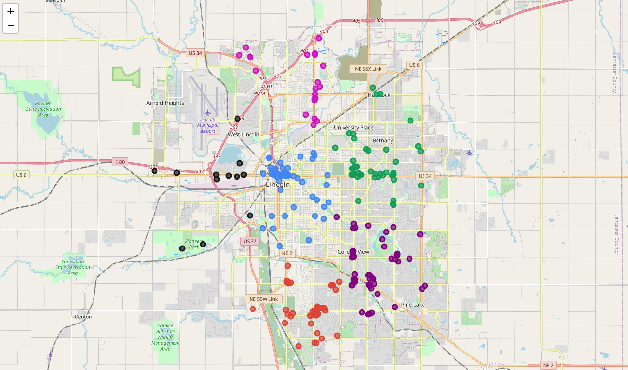 - -# Investigate Clusters - -Now that we have figured out our clusters, let's do a little more -analysis to provide more insight into the clusters. With the information -below, we can see which clusters are more popular for businesses and -which are less popular. The results below show us that clusters 0 -through 3 are popular, while clusters 4 and 5 are not very popular at -all. - -```python -# Show how many venues are in each cluster -color_names = ['Dark Green', 'Red', 'Blue', 'Purple', 'Pink', 'Black'] -for x in range(0,6): - print("Color of Cluster", x, ":", color_names[x]) - print("Venues found in Cluster", x, ":", nearby_venues.loc[nearby_venues['Cluster Labels'] == x, nearby_venues.columns[:]].shape[0]) - print("---") -``` - -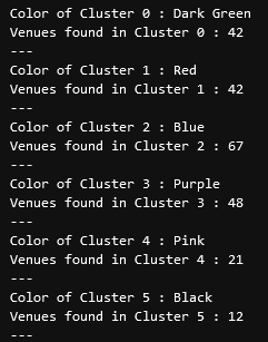 - -Our last piece of analysis is to summarize the categories of businesses -within each cluster. With these results, we can clearly see that -restaurants, coffee shops, and grocery stores are the most popular. - -```python -# Calculate how many venues there are in each category -# Sort from largest to smallest -temp_df = nearby_venues.drop(columns=['name', 'lat', 'lng']) - -cluster0_grouped = temp_df.loc[temp_df['Cluster Labels'] == 0].groupby(['categories']).count().sort_values(by='Cluster Labels', ascending=False) -cluster1_grouped = temp_df.loc[temp_df['Cluster Labels'] == 1].groupby(['categories']).count().sort_values(by='Cluster Labels', ascending=False) -cluster2_grouped = temp_df.loc[temp_df['Cluster Labels'] == 2].groupby(['categories']).count().sort_values(by='Cluster Labels', ascending=False) -cluster3_grouped = temp_df.loc[temp_df['Cluster Labels'] == 3].groupby(['categories']).count().sort_values(by='Cluster Labels', ascending=False) -cluster4_grouped = temp_df.loc[temp_df['Cluster Labels'] == 4].groupby(['categories']).count().sort_values(by='Cluster Labels', ascending=False) -cluster5_grouped = temp_df.loc[temp_df['Cluster Labels'] == 5].groupby(['categories']).count().sort_values(by='Cluster Labels', ascending=False) - -# show how many venues there are in each cluster (> 1) -with pd.option_context('display.max_rows', None, 'display.max_columns', None): - print("\n\n", "Cluster 0:", "\n", cluster0_grouped.loc[cluster0_grouped['Cluster Labels'] > 1]) - print("\n\n", "Cluster 1:", "\n", cluster1_grouped.loc[cluster1_grouped['Cluster Labels'] > 1]) - print("\n\n", "Cluster 2:", "\n", cluster2_grouped.loc[cluster2_grouped['Cluster Labels'] > 1]) - print("\n\n", "Cluster 3:", "\n", cluster3_grouped.loc[cluster3_grouped['Cluster Labels'] > 1]) - print("\n\n", "Cluster 4:", "\n", cluster4_grouped.loc[cluster4_grouped['Cluster Labels'] > 1]) - print("\n\n", "Cluster 5:", "\n", cluster5_grouped.loc[cluster5_grouped['Cluster Labels'] > 1]) -``` - -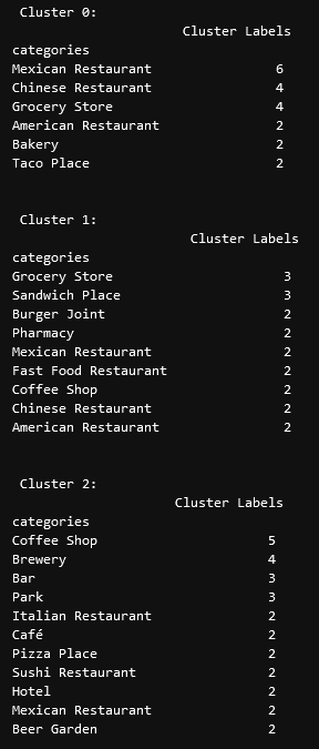 - -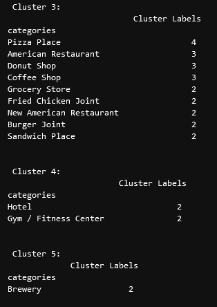 - -# Discussion - -In this project, we gathered location data for Lincoln, Nebraska, USA -and clustered the data using the k-means algorithm in order to identify -the unique clusters of businesses in Lincoln. Through these actions, we -found that there are six unique business clusters in Lincoln and that -two of the clusters are likely unsuitable for investors. The remaining -four clusters have a variety of businesses, but are largely dominated by -restaurants and grocery stores. - -Using this project, investors can now make more informed decisions when -deciding the location and category of business in which to invest. - -Further studies may involve other attributes for business locations, -such as population density, average wealth across the city, or crime -rates. In addition, further studies may include additional location data -and businesses by utilizing multiple sources, such as Google Maps and -OpenStreetMap. |