path: root/content/blog/2020-07-26-business-analysis.md

+++
date = 2020-07-26
title = "Algorithmically Analyzing Local Businesses "
description = ""
draft = false
+++

# Background Information

This project aims to help investors learn more about a random city in
order to determine optimal locations for business investments. The data
used in this project was obtained using Foursquare\'s developer API.

Fields include:

-   Venue Name
-   Venue Category
-   Venue Latitude
-   Venue Longitude

There are 232 records found using the center of Lincoln as the area of
interest with a radius of 10,000.

# Import the Data

The first step is the simplest: import the applicable libraries. We will
be using the libraries below for this project.

``` python
# Import the Python libraries we will be using
import pandas as pd
import requests
import folium
import math
import json
from pandas.io.json import json_normalize
from sklearn.cluster import KMeans
```

To begin our analysis, we need to import the data for this project. The
data we are using in this project comes directly from the Foursquare
API. The first step is to get the latitude and longitude of the city
being studied (Lincoln, NE) and setting up the folium map.

``` python
# Define the latitude and longitude, then map the results
latitude = 40.806862
longitude = -96.681679
map_LNK = folium.Map(location=[latitude, longitude], zoom_start=12)

map_LNK
```

![Blank
Map](https://img.cleberg.net/blog/20200726-ibm-data-science/01_blank_map-min.png)

Now that we have defined our city and created the map, we need to go get
the business data. The Foursquare API will limit the results to 100 per
API call, so we use our first API call below to determine the total
results that Foursquare has found. Since the total results are 232, we
perform the API fetching process three times (100 + 100 + 32 = 232).

``` python
# Foursquare API credentials
CLIENT_ID = 'your-client-id'
CLIENT_SECRET = 'your-client-secret'
VERSION = '20180604'

# Set up the URL to fetch the first 100 results
LIMIT = 100
radius = 10000
url = 'https://api.foursquare.com/v2/venues/explore?&client_id={}&client_secret={}&v={}&ll={},{}&radius={}&limit={}'.format(
    CLIENT_ID,
    CLIENT_SECRET,
    VERSION,
    latitude,
    longitude,
    radius,
    LIMIT)

# Fetch the first 100 results
results = requests.get(url).json()

# Determine the total number of results needed to fetch
totalResults = results['response']['totalResults']
totalResults

# Set up the URL to fetch the second 100 results (101-200)
LIMIT = 100
offset = 100
radius = 10000
url2 = 'https://api.foursquare.com/v2/venues/explore?&client_id={}&client_secret={}&v={}&ll={},{}&radius={}&limit={}&offset={}'.format(
    CLIENT_ID,
    CLIENT_SECRET,
    VERSION,
    latitude,
    longitude,
    radius,
    LIMIT,
    offset)

# Fetch the second 100 results (101-200)
results2 = requests.get(url2).json()

# Set up the URL to fetch the final results (201 - 232)
LIMIT = 100
offset = 200
radius = 10000
url3 = 'https://api.foursquare.com/v2/venues/explore?&client_id={}&client_secret={}&v={}&ll={},{}&radius={}&limit={}&offset={}'.format(
    CLIENT_ID,
    CLIENT_SECRET,
    VERSION,
    latitude,
    longitude,
    radius,
    LIMIT,
    offset)

# Fetch the final results (201 - 232)
results3 = requests.get(url3).json()
```

# Clean the Data

Now that we have our data in three separate dataframes, we need to
combine them into a single dataframe and make sure to reset the index so
that we have a unique ID for each business. The
`get~categorytype~` function below will pull the categories
and name from each business\'s entry in the Foursquare data
automatically. Once all the data has been labeled and combined, the
results are stored in the `nearby_venues` dataframe.

``` python
# This function will extract the category of the venue from the API dictionary
def get_category_type(row):
    try:
        categories_list = row['categories']
    except:
        categories_list = row['venue.categories']

    if len(categories_list) == 0:
        return None
    else:
        return categories_list[0]['name']

# Get the first 100 venues
venues = results['response']['groups'][0]['items']
nearby_venues = json_normalize(venues)

# filter columns
filtered_columns = ['venue.name', 'venue.categories', 'venue.location.lat', 'venue.location.lng']
nearby_venues = nearby_venues.loc[:, filtered_columns]

# filter the category for each row
nearby_venues['venue.categories'] = nearby_venues.apply(get_category_type, axis=1)

# clean columns
nearby_venues.columns = [col.split(".")[-1] for col in nearby_venues.columns]

---

# Get the second 100 venues
venues2 = results2['response']['groups'][0]['items']
nearby_venues2 = json_normalize(venues2) # flatten JSON

# filter columns
filtered_columns2 = ['venue.name', 'venue.categories', 'venue.location.lat', 'venue.location.lng']
nearby_venues2 = nearby_venues2.loc[:, filtered_columns]

# filter the category for each row
nearby_venues2['venue.categories'] = nearby_venues2.apply(get_category_type, axis=1)

# clean columns
nearby_venues2.columns = [col.split(".")[-1] for col in nearby_venues.columns]
nearby_venues = nearby_venues.append(nearby_venues2)

---

# Get the rest of the venues
venues3 = results3['response']['groups'][0]['items']
nearby_venues3 = json_normalize(venues3) # flatten JSON

# filter columns
filtered_columns3 = ['venue.name', 'venue.categories', 'venue.location.lat', 'venue.location.lng']
nearby_venues3 = nearby_venues3.loc[:, filtered_columns]

# filter the category for each row
nearby_venues3['venue.categories'] = nearby_venues3.apply(get_category_type, axis=1)

# clean columns
nearby_venues3.columns = [col.split(".")[-1] for col in nearby_venues3.columns]

nearby_venues = nearby_venues.append(nearby_venues3)
nearby_venues = nearby_venues.reset_index(drop=True)
nearby_venues
```

![Clean
Data](https://img.cleberg.net/blog/20200726-ibm-data-science/02_clean_data-min.png)

# Visualize the Data

We now have a complete, clean data set. The next step is to visualize
this data onto the map we created earlier. We will be using folium\'s
`CircleMarker()` function to do this.

``` python
# add markers to map
for lat, lng, name, categories in zip(nearby_venues['lat'], nearby_venues['lng'], nearby_venues['name'], nearby_venues['categories']):
    label = '{} ({})'.format(name, categories)
    label = folium.Popup(label, parse_html=True)
    folium.CircleMarker(
        [lat, lng],
        radius=5,
        popup=label,
        color='blue',
        fill=True,
        fill_color='#3186cc',
        fill_opacity=0.7,
        ).add_to(map_LNK)

map_LNK
```

\![Initial data
map](https://img.cleberg.net/blog/20200726-ibm-data-science/03_data_map-min.png)

# Clustering: *k-means*

To cluster the data, we will be using the *k-means* algorithm. This
algorithm is iterative and will automatically make sure that data points
in each cluster are as close as possible to each other, while being as
far as possible away from other clusters.

However, we first have to figure out how many clusters to use (defined
as the variable *\'k\'*). To do so, we will use the next two functions
to calculate the sum of squares within clusters and then return the
optimal number of clusters.

``` python
# This function will return the sum of squares found in the data
def calculate_wcss(data):
    wcss = []
    for n in range(2, 21):
        kmeans = KMeans(n_clusters=n)
        kmeans.fit(X=data)
        wcss.append(kmeans.inertia_)

    return wcss

# Drop 'str' cols so we can use k-means clustering
cluster_df = nearby_venues.drop(columns=['name', 'categories'])

# calculating the within clusters sum-of-squares for 19 cluster amounts
sum_of_squares = calculate_wcss(cluster_df)

# This function will return the optimal number of clusters
def optimal_number_of_clusters(wcss):
    x1, y1 = 2, wcss[0]
    x2, y2 = 20, wcss[len(wcss)-1]

    distances = []
    for i in range(len(wcss)):
        x0 = i+2
        y0 = wcss[i]
        numerator = abs((y2-y1)*x0 - (x2-x1)*y0 + x2*y1 - y2*x1)
        denominator = math.sqrt((y2 - y1)**2 + (x2 - x1)**2)
        distances.append(numerator/denominator)

    return distances.index(max(distances)) + 2

# calculating the optimal number of clusters
n = optimal_number_of_clusters(sum_of_squares)
```

Now that we have found that our optimal number of clusters is six, we
need to perform k-means clustering. When this clustering occurs, each
business is assigned a cluster number from 0 to 5 in the dataframe.

``` python
# set number of clusters equal to the optimal number
kclusters = n

# run k-means clustering
kmeans = KMeans(n_clusters=kclusters, random_state=0).fit(cluster_df)

# add clustering labels to dataframe
nearby_venues.insert(0, 'Cluster Labels', kmeans.labels_)
```

Success! We now have a dataframe with clean business data, along with a
cluster number for each business. Now let\'s map the data using six
different colors.

``` python
# create map with clusters
map_clusters = folium.Map(location=[latitude, longitude], zoom_start=12)
colors = ['#0F9D58', '#DB4437', '#4285F4', '#800080', '#ce12c0', '#171717']

# add markers to the map
for lat, lng, name, categories, cluster in zip(nearby_venues['lat'], nearby_venues['lng'], nearby_venues['name'], nearby_venues['categories'], nearby_venues['Cluster Labels']):
    label = '[{}] {} ({})'.format(cluster, name, categories)
    label = folium.Popup(label, parse_html=True)
    folium.CircleMarker(
        [lat, lng],
        radius=5,
        popup=label,
        color=colors[int(cluster)],
        fill=True,
        fill_color=colors[int(cluster)],
        fill_opacity=0.7).add_to(map_clusters)

map_clusters
```

![Clustered
Map](https://img.cleberg.net/blog/20200726-ibm-data-science/04_clusters-min.png)

# Investigate Clusters

Now that we have figured out our clusters, let\'s do a little more
analysis to provide more insight into the clusters. With the information
below, we can see which clusters are more popular for businesses and
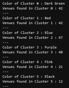
which are less popular. The results below show us that clusters 0
through 3 are popular, while clusters 4 and 5 are not very popular at
all.

``` python
# Show how many venues are in each cluster
color_names = ['Dark Green', 'Red', 'Blue', 'Purple', 'Pink', 'Black']
for x in range(0,6):
    print("Color of Cluster", x, ":", color_names[x])
    print("Venues found in Cluster", x, ":", nearby_venues.loc[nearby_venues['Cluster Labels'] == x, nearby_venues.columns[:]].shape[0])
    print("---")
```

![Venues per
Cluster](https://img.cleberg.net/blog/20200726-ibm-data-science/05_venues_per_cluster-min.png)

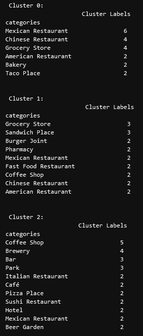
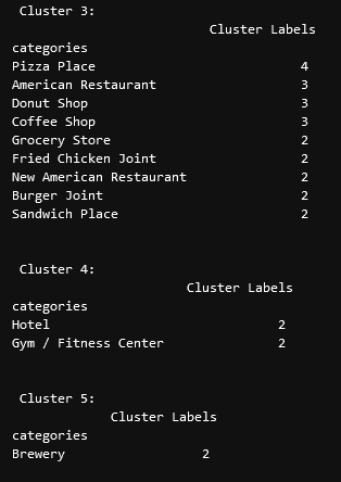
Our last piece of analysis is to summarize the categories of businesses
within each cluster. With these results, we can clearly see that
restaurants, coffee shops, and grocery stores are the most popular.

``` python
# Calculate how many venues there are in each category
# Sort from largest to smallest
temp_df = nearby_venues.drop(columns=['name', 'lat', 'lng'])

cluster0_grouped = temp_df.loc[temp_df['Cluster Labels'] == 0].groupby(['categories']).count().sort_values(by='Cluster Labels', ascending=False)
cluster1_grouped = temp_df.loc[temp_df['Cluster Labels'] == 1].groupby(['categories']).count().sort_values(by='Cluster Labels', ascending=False)
cluster2_grouped = temp_df.loc[temp_df['Cluster Labels'] == 2].groupby(['categories']).count().sort_values(by='Cluster Labels', ascending=False)
cluster3_grouped = temp_df.loc[temp_df['Cluster Labels'] == 3].groupby(['categories']).count().sort_values(by='Cluster Labels', ascending=False)
cluster4_grouped = temp_df.loc[temp_df['Cluster Labels'] == 4].groupby(['categories']).count().sort_values(by='Cluster Labels', ascending=False)
cluster5_grouped = temp_df.loc[temp_df['Cluster Labels'] == 5].groupby(['categories']).count().sort_values(by='Cluster Labels', ascending=False)

# show how many venues there are in each cluster (> 1)
with pd.option_context('display.max_rows', None, 'display.max_columns', None):
    print("\n\n", "Cluster 0:", "\n", cluster0_grouped.loc[cluster0_grouped['Cluster Labels'] > 1])
    print("\n\n", "Cluster 1:", "\n", cluster1_grouped.loc[cluster1_grouped['Cluster Labels'] > 1])
    print("\n\n", "Cluster 2:", "\n", cluster2_grouped.loc[cluster2_grouped['Cluster Labels'] > 1])
    print("\n\n", "Cluster 3:", "\n", cluster3_grouped.loc[cluster3_grouped['Cluster Labels'] > 1])
    print("\n\n", "Cluster 4:", "\n", cluster4_grouped.loc[cluster4_grouped['Cluster Labels'] > 1])
    print("\n\n", "Cluster 5:", "\n", cluster5_grouped.loc[cluster5_grouped['Cluster Labels'] > 1])
```

![Venues per Cluster, pt.
1](https://img.cleberg.net/blog/20200726-ibm-data-science/06_categories_per_cluster_pt1-min.png)

![Venues per Cluster, pt.
2](https://img.cleberg.net/blog/20200726-ibm-data-science/07_categories_per_cluster_pt2-min.png)

# Discussion

In this project, we gathered location data for Lincoln, Nebraska, USA
and clustered the data using the k-means algorithm in order to identify
the unique clusters of businesses in Lincoln. Through these actions, we
found that there are six unique business clusters in Lincoln and that
two of the clusters are likely unsuitable for investors. The remaining
four clusters have a variety of businesses, but are largely dominated by
restaurants and grocery stores.

Using this project, investors can now make more informed decisions when
deciding the location and category of business in which to invest.

Further studies may involve other attributes for business locations,
such as population density, average wealth across the city, or crime
rates. In addition, further studies may include additional location data
and businesses by utilizing multiple sources, such as Google Maps and
OpenStreetMap.